Half lives: counting backwards
|
Half lives: counting backwards |
Introduction to rate |
||||||||||||||||||||
The climate has changed in the past and is changing now. The effects of climate change are often a result of the rate (speed) of the change, so understanding rates is an important part of climate science. The changes may involve chemical reactions—changes of reactant(s) to product(s). For example, the expression, A→B, represents reactant A changing to product B. In many such reactions, the rate at which A reacts (disappears to form B) is directly proportional to the amount of A left to react, that is, - rate of disappearance of A = k[A]. Here, k is a proportionality constant (called the “rate constant”) and [A] is the amount (concentration) of A remaining unreacted at the time the rate is determined during the reaction. The negative sign is included because we want rates to be positive quantities, but A is going away, so its change will be negative and the negative sign compensates for that. Reactions that follow this pathway are called “first order reactions”, because the rate depends on [A] with an exponent of one (not zero or two, which characterize other reactions). A common example of a first order reaction is the decay of radioactive nuclei (used, for example, to date objects from the past). Many reactions are first order (or can be analyzed as pseudo first order). A mathematical analysis of the rate equation above for first order reactions leads to this equation: |
||||||||||||||||||||
A. Rate of change counting analogy |
||||||||||||||||||||
|
||||||||||||||||||||
| Procedure | ||||||||||||||||||||
Shake the bag of candies to mix the sample thoroughly, and then spill the candies out on a flat surface. If you plan to eat the M&Ms later, pour them onto clean paper towels or other clean paper. Put all of the M&Ms whose “m” is showing into a clean paper cup. (Look carefully—it can be difficult to see the “m” on the light colored candies.) Label this cup #1. Place the “unselected” candies, those with the “m” face down, back in the bag. Repeat the shaking, spilling, and selecting. Each time you repeat the process put the removed candies into a new clean paper cup (numbers 2, 3, … ). Stop when you have about 13±2 M&Ms remaining “unselected”. Check these and discard (or eat) any that do not have an “m” on either side. Count the number remaining on the surface (after throwing away the “defective” candies), and record the number below as the number remaining at the end. Also record the total number of spills (equal to the number of the last cup). |
||||||||||||||||||||
| Observations | ||||||||||||||||||||
 |
||||||||||||||||||||
| Analysis | ||||||||||||||||||||
1.
|
Assuming that each M&M has an equal probability of ending up with the “m” up or “m” down, what fraction of the candies should remain after each spill? Give the reasoning for your answer. (Of course, this assumes that each M&M actually has one side with an “m” and one without, which is why you removed any “defective” candies.) |
|||||||||||||||||||
2.
|
Explain how each spill represents a half-life for “decay” of the original sample of M&Ms. |
|||||||||||||||||||
3.
|
Explain how you could estimate the number of M&Ms in the original sample using just the number of M&Ms remaining at the end, together with the number of spills. |
|||||||||||||||||||
4.
|
Use the method you described in item 3, to estimate the number of M&Ms you started with. |
|||||||||||||||||||
5.
|
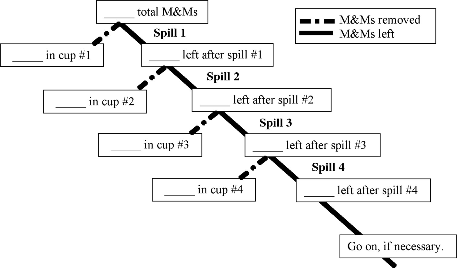
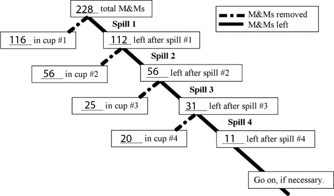
Count the M&Ms in each cup, and use this information, plus number of M&Ms left after the last spill, to fill in the blanks in this diagram. How does the experimental value for the total number of M&Ms in your sample compare to the number you calculated in item 4? What explanation might you give for any difference? |
|||||||||||||||||||
|
||||||||||||||||||||
6.
|
Use the data from the previous diagram to calculate the decimal fraction of the original number of M&Ms that were replaced in the bag after each spill, including the fraction left after the final spill, and record the results in this table. E.g., the entry in the cell under “1” will be:
|
|||||||||||||||||||
7.
|
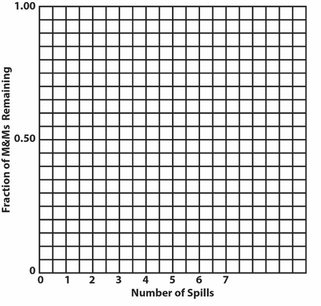
Plot a graph of these data on the following grid. |
|||||||||||||||||||
B. Half-life and radioactive decay |
||||||||||||||||||||
The half-life of a radioactive substance is defined as the time required for half of the sample to decay. |
||||||||||||||||||||
8.
|
What fraction of a radioactive sample remains after one half-life? Explain. |
|||||||||||||||||||
9.
|
What fraction remains after two half-lives? Explain. |
|||||||||||||||||||
10.
|
What fraction remains after three half-lives? Explain. |
|||||||||||||||||||
11.
|
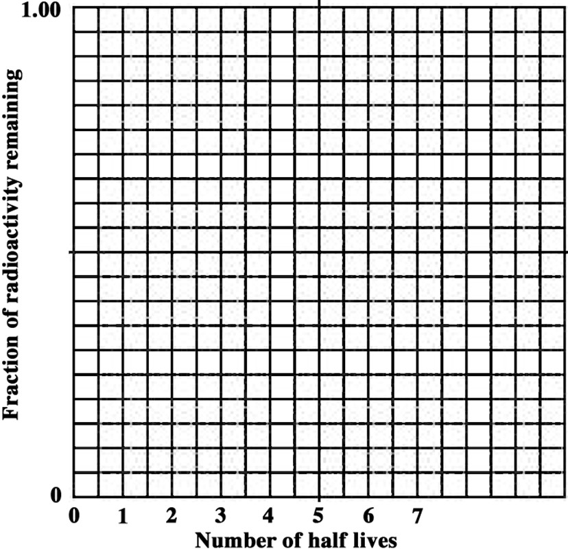
On the following grid, plot a graph showing the fraction of a radioactive sample remaining as a function of the number of half-lives elapsed. Include at least 5 half-lives. |
|||||||||||||||||||
12.
|
In what way(s) is the half-life graph similar to the graph of the M&M “reaction”? |
|||||||||||||||||||
13.
|
Describe how the example of the M&M simulation is related to the concept of half-life. |
|||||||||||||||||||
| Check your understanding | ||||||||||||||||||||
14.
|
|
|||||||||||||||||||
|
||||||||||||||||||||
|
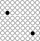
(a) How many radioactive nuclei were initially present in the sample? Explain your response. (b) How many radioactive nuclei will be present after one half-life? after two? etc. Explain your responses. (c) The figure represents the sample after 250 days. What is the half-life of the radioactive isotope? Describe the sample 100 days earlier. Explain your responses. (d) Describe the sample 75 days earlier and explain your answer. |
|||||||||||||||||||
C. First-order reactions |
||||||||||||||||||||
The analysis in item 14(c) is based on an integral number of half-lives. The analysis in item 14(d) is based on an interpolation of the fraction remaining between half-lives. An analytical procedure explicitly involving time would be more desirable, more general, and more applicable to item 14(d). |
||||||||||||||||||||
15.
|
Consider, again, the M&Ms activity. Let N0 be the total number M&Ms and Nn be the number remaining after n spills. Assuming the ideal case presented in item 1, develop an equation that will predict Nn as a function of n and N0. |
|||||||||||||||||||
16.
|
The fraction of M&Ms remaining after n half-lives, fn, is Nn/N0. Rearrange your equation from item 15 to give the fraction remaining as a function of n. |
|||||||||||||||||||
17.
|
Your equations from items 15 and 16 are applicable to any first order reaction, that is, one where an initial amount (concentration) of reactant decays over time to a smaller amount (concentration) that can be characterized by how many half-lives have elapsed. The number of half-lives is equal to the amount of time the reaction has been going on, t, divided by the half-life for the reaction, τ (Greek lower case tau is usually used to designate half-life). Thus, n = t/τ. Substitute this ratio for n in your equation from item 16 and take the logarithm (base e, i.e., ln) of both sides of this equation. |
|||||||||||||||||||
18.
|
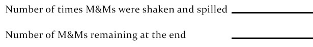
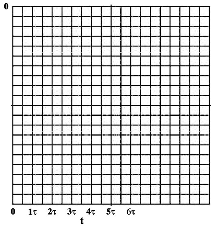
Assume that each spill in the M&Ms activity corresponds to one half-life, τ, and that t is the time elapsed during the process. Use the data from your table in item 6 to plot ln fn (the logarithm of the fraction of M&Ms remaining after n half-lives) as a function of t (in units of τ) on the left-hand grid. |
|||||||||||||||||||
  |
||||||||||||||||||||
19.
|
Is your plot consistent with the logarithmic equation in item 17? Explain why or why not. Hint: Consider the shape of the curve and, if possible, its slope. |
|||||||||||||||||||
20. |
Another approach to describing first order reactions is to use calculus and write the rate law as, where [A] is the amount (concentration) of the reactant. Separating the variables and integrating gives: |
|||||||||||||||||||
21.
|
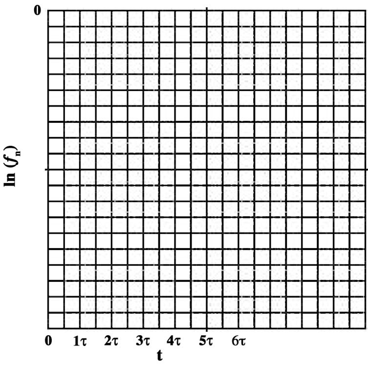
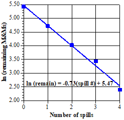
Rearranging the integrated rate law gives, ln[At] = –kt + ln[A0], so a plot of ln[At] as a function of t should be a straight line. Use the right-hand grid above to show that this equation fits the data in item 5 for the M&Ms activity. |
|||||||||||||||||||
22.
|
Here are a couple example problems whose solutions use the relationship between first order reactions and half-life. (a) All living plants contain about the same percentage of carbon-14. When the plant dies, no more carbon-14 is added; the isotope decays by beta particle emission with a half-life of 5730 years. A sample of wood from an archaeological excavation had about 20% as much carbon-14 as living wood. About how old is the sample? Explain your response. (Given a remaining fraction and the half-life, the problem is to find the time elapsed since the decay began.) (b) Apply this relationship to item 14(d) and explain possible limitations on its use. (Given an elapsed time and the half-life, the problem is to find the fraction remaining.) |
|||||||||||||||||||
 |
||||||||||||||||||||
Instructor/presenter notes |
||||||||||||||||||||
Expected/possible responses to the items in the activity worksheet are: |
||||||||||||||||||||
Part A |
||||||||||||||||||||
1. |
If, in a perfect world, there is equal probability of an M&M landing “m” up or “m” down, exactly half the M&Ms would land “m” up and half “m” down. Since the world is not perfect and we are working with relatively small numbers, the actual results will only fortuitously be exactly half and half. See suggestions at the end of these responses to the number items for a possible way to improve statistics. |
|||||||||||||||||||
2. |
Since half of the original amount of a sample decays/reacts during a half-life, one spill of a sample of the M&Ms, which (theoretically) results in half of them being removed, is like a half-life in its effect on the sample. The idea, spill equivalent to half-life, recurs often below. |
|||||||||||||||||||
3. |
Depending on the backgrounds of the students, there may be different ways to work back from the number of remaining M&Ms to the size of the original sample. The most common correct approach uses the idea of equal probability at each spill to double the number remaining to get the previous amount and continuing the doubling until the number of doublings corresponds to the number of spills. This is equivalent to multiplying the number remaining by 2number of spills, which sometimes also comes up when students have enough background in probability and think about applying it. |
|||||||||||||||||||
4. |
Item 5 gives an example of data from this Activity, for which 11 M&Ms remain after four spills. Assuming that the method from item 3 is doubling, these data give 176 (= 11•24) as the starting number of M&Ms. Most trials with this Activity will give 13 ± 2 remaining M&Ms after four spills, so the results for this backwards count will be 176, 192, 208, 224, or 240. The occasional outlier is a trial that gives more than 15 remaining M&Ms after four spills, so a fifth spill is done that almost always results in fewer than 11 M&Ms remaining. The backwards count is done in exactly the same way with 32 (= 25) as the doubling factor. |
|||||||||||||||||||
5. |
The data from the trial of the Activity reported on this diagram are used for the rest of this discussion. The calculated total number of M&Ms from these data, 176 (item 4), is almost 25% smaller than the actual number, 228. A result like this does not inspire confidence in the “counting backwards” method, but requires a discussion of the unreliability of the statistics of small samples. The scatter of results among several groups in a class should provide background for a productive discussion. A group whose calculated value is close to the experimental value should be encouraged to consider how fortunate (lucky) they were not to have one fewer or one more remaining M&M than they had, for example. |
|||||||||||||||||||
|
||||||||||||||||||||
6. |
Example chart using data from the diagram in item 5. |
|||||||||||||||||||
|
||||||||||||||||||||
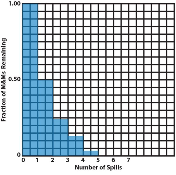
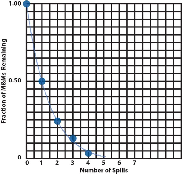
7. |
These are two ways to plot the data from item 6, a bar graph and a scatter plot (or an x-y plot). A bar graph is useful when the independent variable represents a discrete set of categories whose dependent-variable values are to be compared. Here, the independent variable is the spill number and their dependent variable is the remaining fraction of M&Ms. This plot looks like a staircase with decreasing height risers from one step to the next. In a scatter plot, the independent variable varies continuously (or might be imagined to do so). The mathematical pattern of change of the dependent-variable values can be used to interpolate between the discreet plotted points to determine values that haven’t been measured. This is illustrated here by the lightly drawn curve that leads your eye from one point to the next. The curve is calculated by assuming there is an underlying mathematically continuous function that represents the changing values of the dependent variable and finding the function that best fits the data. In this particular case (the M&M activity), intermediate values make no sense, because the analogy is only to half-life without regard to what is happening between spills. But, for actual reactions occurring continuously, this analysis is useful, as we will see below. |
|||||||||||||||||||
  |
||||||||||||||||||||
Part B |
||||||||||||||||||||
8. |
All the radioactive nuclei in the original sample are present at the start, so the fraction present is 1.000. Half of the original radioactive nuclei decay during the first half life, so the fraction remaining undecayed will be 1.000•(1/2) = 0.500. |
|||||||||||||||||||
9. |
The second half-life begins with half of the original sample left to decay (the 0.500 from item 8). Half of this decays during the second half-life, so the fraction remaining unreacted will be 0.500•(1/2) = 0.250, that is, a quarter of the original sample. One-quarter (0.250) of the original sample remains after the second half-life. |
|||||||||||||||||||
10. |
Half of the unreacted nuclei left after the second half-life decay during the third half-life, leaving 0.250•(1/2) = (1/4)•(1/2) = 1/8 = 0.125, one-eighth of the original sample. One-eighth (0.125) of the original sample remains after the third half-life. Continuing this process of halving for each half-life leads to the results in this table. |
|||||||||||||||||||
|
||||||||||||||||||||
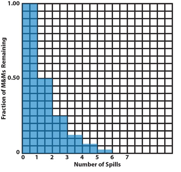
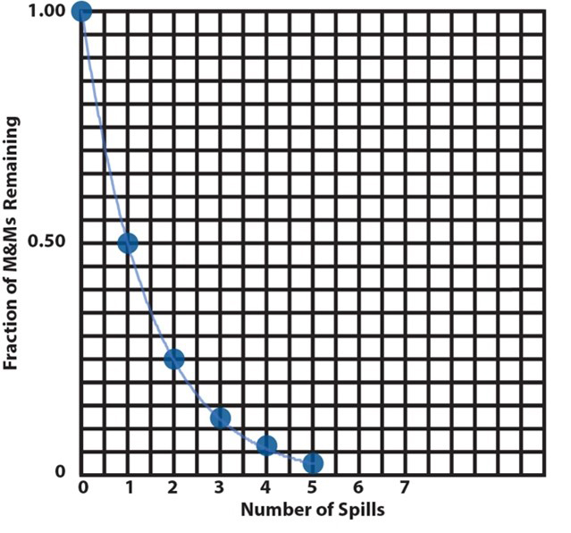
11. |
As in item 7, two plots, a bar chart and a scatter plot, of the data in the table are shown here. If all participant groups have calculated the half-lives correctly (items 8, 9, and 10), plots should all be the same. For this example, representing an actual radioactive sample decay, the continuous exponential curve drawn through the plotted points has physical significance. A radioactive sample decays continuously by a first order process that follows a time course represented by the curve on the plot. At any time during the decay, the fraction of nuclei remaining unreacted is the fraction value of the curve corresponding to that time. Conversely, if we know the fraction of reaction that has occurred, we can find the time that has elapsed since the reaction began. The elapsed time for any fraction of the reaction is the time value of the curve at that fraction. We will see below how to find the amount of a reactant remaining unreacted or the elapsed time for a given fraction of reaction without having to read a graph. |
|||||||||||||||||||
  |
||||||||||||||||||||
12. |
Except in rare random “pathological” cases, the plots from the M&M analogy and the half-life calculations should look very much alike. If bar charts are made, participants should note the similar staircase appearance with decreasing jumps from one step to another, especially noticeable for the first two steps and likely to be about the same for both plots. If scatter plots are made, participants should note the similar shape of the “curve” represented by the points with the precipitous decrease for the early part of the plot and the much gentler decrease toward the later (lower) part of the plots. Participants may see other similarities as well and these can be starting points for further discussion of the meaning of the data or of extraneous distractors that interfere with interpretation of the plots. |
|||||||||||||||||||
13. |
During a half-life, one-half of a sample reacts, leaving half of the sample unreacted. For the M&M activity, one half of the M&Ms spilled should, in theory, land “m” up and the other half “m” down. Consecutive half-lives or consecutive spills should lead to the same descending series of remaining fractions of the original sample. Comparison of these plots is designed to exemplify this correlation between half-lives and spills in the M&M analogy and make the spills equal half-lives idea more concrete. |
|||||||||||||||||||
14. |
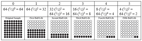
(a) The sample shown has 64 circles, each representing either a radioactive isotope or the product of its decay. Since the sample originally contained only radioactive isotopes, there were 64 radioactive nuclei in the original sample. (b) During each half-life, half of the beginning radioactive nuclei decay. This table shows the results for five half-lives of this sample. The top row of the table is the half-life number, the second row is the calculation of the number of nuclei left unreacted at the end of each half-life, and the third row are easy-to-count pictorial representations of the sample after each half-life. (Note: any number raised to the zeroth power is one, so (1/2)0 = 1.) |
|||||||||||||||||||
 |
||||||||||||||||||||
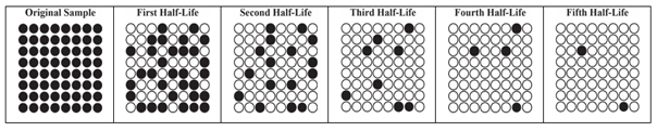
It takes five half-lives for the sample to decay from 64 to 2 radioactive nuclei. The pictorial representations in this table could be misleading, if they leave an impression that the nuclei decay in this sort of patterned way. Here is a series of pictures that better represent the randomness of the decay process, but are not as easy to count for the first couple half-lives. |
||||||||||||||||||||
 |
||||||||||||||||||||
(c) Another possible approach, without going through all the above calculations or pictures, is to start with the fact that an original sample of 64 radioactive nuclei had decayed until only two were left. That is, the fraction remaining is 1/32 (= 2/64), which is five half-lives, (1/2)5. Five half-lives must have elapsed since the decay began 250 days ago. If five half-lives is 250 days, one half-life must be 50 days (250/5). 100 days before would be two half-lives previous or three half-lives from the start. This would leave 1/8 (= (1/2)3) of the original sample at that time, that is, 8 undecayed [= (64 undecayed)(1/8) = 8 undecayed]. A third possible approach is to work backwards as with the estimate of the number of M&Ms before counting them. One half-life ago, 4 radioactive. Two half-lives ago, 8 radioactive. Three half-lives ago, 16 radioactive. Four half-lives ago, 32 radioactive. Five half-lives ago, 64 (all) radioactive, making five total half-lives since the original sample. (d) At 75 days earlier the sample is between three and four half-lives decayed, so the number of undecayed nuclei remaining will be between 8 and 4. It is tempting to think that 6 will remain because we are right in the middle of a half-life. However, the decay is exponential, so more than half the undecayed nuclei will have decayed. In this oversimplified case, the best we can say is that between 2 and 3 of the nuclei will have decayed (leaving 6 or 5 still undecayed) and we can’t tell exactly what would be observed in this tiny sample where the simple statistics don’t really apply. The basic idea is that decay is “continuous” and does not occur in discrete steps as in the M&Ms analogy. (The sample in this problem is represented as a rectangular array, so the total number of initial reactants and decay products is easy to determine. The symbols could just be randomly scattered, but that makes counting more difficult and prone to error. This is a check on understanding half-life, not an assessment of counting ability, and there is no pedagogical reason for making counting difficult.) |
||||||||||||||||||||
Part C |
||||||||||||||||||||
15. |
For every spill, we multiply the starting number by 1/2 to get the number remaining after that spill. After n spills, we will have multiplied the original number of M&Ms n times by 1/2, that is, (1/2)n. Thus, Nn = N0(1/2)n, which we have been using in previous items without writing it in this general form, except in the item 14(b) table above. It might help students to have them look back at items 8, 9, and 10. Writing out the fraction of sample left, in fraction form (1/2, 1/4, and 1/8, respectively) may help them visualize what the numbers (in particular, the denominators) are doing. They can then see that the original times this fraction is the amount remaining and just need to figure out how to express the changing fraction. |
|||||||||||||||||||
16. |
To express the fraction of M&Ms remaining, |
|||||||||||||||||||
17. |
Substituting t/τ for n in the above equation gives: fn = (1/2)n = (1/2)t/τ. Taking the logarithm (base e) of both sides of this equation gives: ln fn = ln (1/2)n = ln (1/2)t/τ. Using the rules of logarithms [ln(x)y = y·ln(x)], take the exponents outside the logarithmic function to give: ln fn = n ln (1/2) = –0.69 n ln ft = (t/τ) ln (1/2) = –0.69 (t/τ) These two equations are equivalent, because n = t/τ. The first focuses attention on the number of half-lives, so the fraction is written with a subscript n. The second focuses on the time the reaction has been going on, so the fraction is written with a subscript t. The equations show that plots of ln fn vs. n and ln ft vs. (t/τ), for first order reactions, should be straight lines with a slope of ln (1/2) = –0.69. Do the M&M results fit this criterion for first order decay? |
|||||||||||||||||||
18.
|
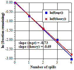
The time units, 0, 1τ, 2τ, etc, on the suggested graph correspond to number of spills. 0, 1, 2, etc. This figure is a graph of the experimental data from item 6 compared to the theoretical half-life data from item 10. |
|||||||||||||||||||
 |
||||||||||||||||||||
19.
|
The linearity is very good and the slope is within 5% of the theoretical value, ln (1/2) = –0.69. Student data almost always yield similar results and should give them confidence that the experiment matches the theoretical equation, even though the statistics are not perfect. For cases where the statistics are better, real radioactive decay of macroscopic samples with very large numbers of atoms, for example, theory and experiment match even better, of course. As the sample size grows (for example, if you combine the data into a class, as suggested below), the two plots should look more and more similar. |
|||||||||||||||||||
20.
|
Since [At]/[A0] is the fraction, ft, of the reactant left at time t, we can write The equation relating ft to the half-life, τ, is Setting the two relationships for ln ft equal to one another gives Dividing both sides of this equation by t gives k as a function of τ: This result makes sense in terms of units. From the differential equation, the units of k have to be 1/time and that is how the units come out here. |
|||||||||||||||||||
21.
|
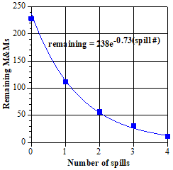
The plots shown so far have been reaction fractions as a function of time, but using the measured experimental data seems more direct. The relationship, ln [At] = –kt + ln [A0], provides a way to do this. To add a bit of context for the ln [At] vs. t plot, we also show a plot of [At] vs. t, with the points fitted by an exponential curve. |
|||||||||||||||||||
  |
||||||||||||||||||||
|
The information from these two plots is identical. In particular, taking the logarithm (base e) of both sides of the exponential curve equation gives the equation for the straight line from the other plot [when the substitution, ln (238) = 5.47, is included]. The slope of this straight line (which is also the constant in the exponent of the exponential equation) is the same as the slope of reaction fraction line in item 18. This has to be the case, because these are just alternative ways of describing the same first order process, so the resulting descriptions must be the same. The most common choice for analyzing a reaction is a logarithmic plot, because deviations from linearity are easy to spot visually. These give a warning that something may be amiss and the assumption of a first order process has to be reassessed. Although very close, the M&M data are not an ideal first order decay, so the slope of the lines here and in item 18 do not give the ideal decay constant, -(1/2) = -0.59. Also, the best statistical straight line or exponential curve does not pass exactly through each experimental point, as is obvious for the last two points. Note (if eagle eyed) that they slightly miss the first point as well. This point represents the starting number of M&Ms, 228 and ln (228) = 5.43, but the curves give 238 and 5.47, that is, intercepts a bit higher on the vertical axis. This is just one more indication that the data do not follow an ideal first order decay—but are very close. This is much like data often obtained for actual reactions in the laboratory, where small uncertainties lead to very good, but not ideal data. |
|||||||||||||||||||
22.
|
Use the relationship, ln ft = –(0.69) (t/τ), to solve both of the problems in this item. (a) The fraction of C-14 remaining, 0.20, and its half-life, 5730 years, are given. Thus: The sample is a little over 13 thousand years old. (b) The half-life for the decay is 50 days [item 14(c)] and the elapsed time since decay began is 175 days (75 days earlier than the 250 days for the final sample shown in the item). Thus: |
|||||||||||||||||||
Other Activities where radioactive isotopes and decay are a basis for understanding more about the planet and its changing climate are Atmospheric CO2: Amount and sources and Earth’s internal energy and atmospheric argon. |
||||||||||||||||||||
|
||||||||||||||||||||
|
||||||||||||||||||||
|
||||||||||||||||||||
To obtain a Word file of this Activity, please fill out this brief form to help us track what is happening to our Workbook. We also encourage you to get in touch if you have an activity or idea for an activity that might add to the Workbook. We want to make this an alive and active document. |
||||||||||||||||||||
| Back to Table of Contents | ||||||||||||||||||||
 |