Atmospheric carbon dioxide amount and source(s)
|
Atmospheric carbon dioxide amount and source(s) |
Background |
|||
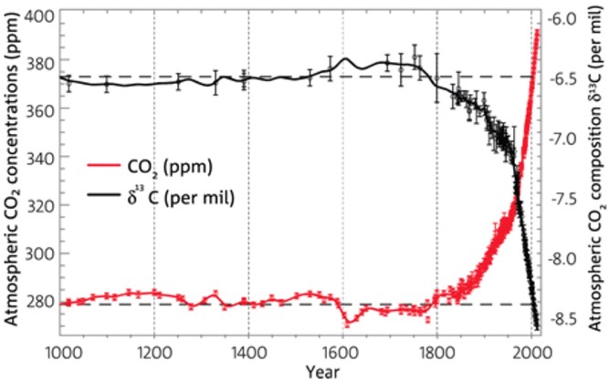
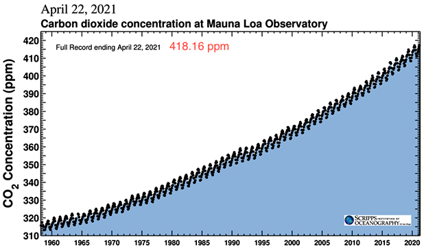
Our instrumental record of the concentration of atmospheric CO2, Figure 1, at the Mauna Loa observatory on the island of Hawaii began in 1958. Previous measurements from gases trapped in ice cores from Greenland and Antarctica show that the concentration was 260 to 280 ppm (parts per million by volume) for at least 10,000 years before 1800, when the concentration began to rise, reached 418 ppm in spring 2021, and continues to rise. Using what we know about the Earth and its atmosphere and further data on the isotopic composition of the CO2, we can find the mass of atmospheric CO2 and a clue to the source of the increase since 1800. |
|||
|
|||
| A. Mass of atmospheric CO2 | |||
The objective of this part is to convert ppm of CO2 to mass of CO2. What we know about the amount of atmospheric CO2 is the number of parts per million in the gas. This is equivalent to the number of moles of CO2 per million moles of gas. Ninety-nine percent of the atmosphere is a mixture of nitrogen and oxygen in about a four-to-one ratio, which gives the gas molecules an average molar mass of 29 g. If we know the mass of the atmosphere, we can calculate the number of moles of gas it contains. The ppm of CO2 gives the number of moles of CO2 and then its mass. Whenever you read a barometer, you are weighing the atmosphere. Appendix A shows how to use atmospheric pressure to find the atmospheric mass, 5.3 x 10¹⁸ kg (=5.3 x 10²¹ g). |
|||
1.
|
How many moles of gas does the atmosphere contain? Explain the reasoning for your response. |
||
2.
|
How many moles are there in one-millionth (10-6) part of the atmosphere? |
||
3.
|
If the atmosphere contains 418 ppm of CO2, how many moles of CO2 is this? |
||
4.
|
The molar mass of CO2 is 44 g. What is the mass (in gigatonnes, 1 Gt = 1015 g) of one part per million, 1 ppm, of CO2 in the atmosphere? Explain the reasoning for your response. |
||
5.
|
About what mass of CO2 has been added to the atmosphere since 1800? Explain the reasoning for your response. |
||
| B. Radiocarbon dating | |||
Three isotopes of carbon, 12C, 13C, and 14C, occur in atmospheric CO2 and many other carbon-containing compounds. Most of the carbon, 98.9%, is 12C with about 1.1% 13C; both are stable isotopes. Carbon-14 is a radioactive isotope (radiocarbon), with a half-life of 5700±30 years (or often as 5730 years, representing a slightly different way of averaging observations). 14C6+ → 14N7+ + 0e-1 (beta decay) Carbon-14 is formed in minuscule amount in the atmosphere by this n,p (neutron,proton) nuclear reaction (with neutrons produced by cosmic radiation). 14N7+ + 1n0 → 14C6+ + 1p+ This natural rate of formation is very nearly constant over time. The atmospheric concentration of 14C, which is a balance between the rate of formation and rate of loss by radioactive decay and uptake by plants, soil, and seas, also remains almost the same. Thus, the amount of atmospheric CO2 formed from this 14C is also about the same all the time. Radiocarbon dating of artifacts from the past depends upon the proportion of 14C in the atmosphere (as 14C in CO2) remaining at least roughly constant over time. If no other factors interfere, the steady state proportion of 14C in the atmosphere should remain the same. Then the plants that use the carbon dioxide in photosynthesis will contain the same proportion of 14C, no matter when the photosynthesis occurs. When the photosynthesis stops (say a reed has been cut down to use in weaving a basket), no more 14C is added. What was in the plant decays with a half-life of about 5730 years, so the amount (in the basket) decreases and dating is based on the fraction that is left, combined with knowledge of how much was there when photosynthesis stopped—that is, the amount from the atmosphere. |
|||
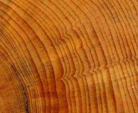
Analysis of 14C in tree rings |
|||
Tree rings, like the ones in Figure 2, can provide a year-by-year look into the environmental history of the tree. Each year a tree adds a new ring on top of the previous ones that are no longer growing. If growth conditions are favorable, the new ring will be relatively thick. If it’s a bad year (too dry, too wet, too cold, etc.), the ring will be rather thin. The rings can be used to count back time from the present year-by-year toward the center of the tree. The tree need not be cut down to get these data. Special borers are available to drill into the tree and extract a cylinder of wood about the diameter of a pencil that can be used to count the rings and analyze them without harming the tree. |
|||
|
|||
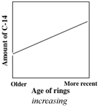
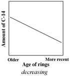
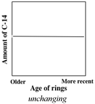
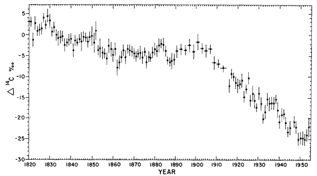
Tree rings provide an excellent way to assess the proportion of 14C in the atmosphere each year from the time the tree started to grow. Each ring adds new material only during the year it grows. The 14C in the older rings represents the proportion of 14C only from the year it was growing. Then it begins to decay with its 5730-year half-life. During the latter part of the 20th century, very sensitive mass spectrometric methods were developed to determine the proportion of 14C in a sample. These make it possible to measure the change in the fraction of 14C in quite small samples over rather short time periods. In about 1980, the 14C proportion (amount) in a set of tree rings spanning the period 1820 to 1954 was analyzed. Figure 3 shows the three possible trends one might expect for the 14C data. (The actual data will, of course, not be nice straight lines—these represent trends.) |
|||
|
|||
6.
|
Based on the previous information, would you expect the trend from older to younger rings to be increasing, decreasing, or unchanging amount of 14C? Clearly explain your choice. |
||
~ Please write your response to item 6 before going on to Part C. ~
|
|||
C. Fossil fuels and atmospheric 14C |
|||
The discussion of radiocarbon dating indicates that, because of its radioactive decay, the older the sample, the lower the fraction of 14C it will contain. Thus, the logical choice in item 6 is that the data will show increasing fractions of 14C, as the tree rings get younger (more recent), Figure 4. |
|||
|
|||
The experimental data are shown in Figure 5. |
|||
|
|||
The data in Figure 5 have been corrected for radiocarbon decay, so, if there were no interfering factor to change the proportion of 14C in the atmosphere, we would expect the plot trend to be basically a horizontal line (with the sort of uncertainties and small fluctuations shown here). Evidently, there is another factor (or factors) at play here to explain the decreasing fraction of 14C with time, especially evident in the first half of the 20th century. (These analyses could not be carried further into the century, because atmospheric testing of nuclear weapons, beginning in the early 50s, added man-made 14C to the atmosphere.) During the 10,000 years before 1800, the concentration of atmospheric CO2 rose from about 260 to 280 ppm, an average increase of about 0.2 ppm per century. From 1800 to present, the concentration has risen about 138 ppm, an average increase of about 60 ppm per century. What has caused this more than 100-fold increased rate of CO2 being added to the atmosphere? Shortly before 1800, the Scottish scientist, James Watt, invented and commercialized the practical steam engine that revolutionized the amount of power available to carry out humanity’s work. Steam engines could be put essentially anywhere a source of power was needed and even put on wheels to move enormous amounts of materials and people from one place to another. The English scientist, Michael Faraday, changed the equation even further by inventing the electric motor and generator. Steam engines could drive generators whose electrical power could be transmitted everywhere, including individual homes, through wires. The Industrial Revolution is aptly named. But it could also be called the Coal Combustion Revolution, since enormous steam power requires enormous production of steam and the largest readily available source of energy to boil the water was coal. As they were discovered and exploited, oil and natural gas have been added to the fuels to be combusted, so now it might be the Fossil Fuel Combustion Revolution (and include internal combustion engines and turbines as well as steam engines). All of this fossil fuel combustion creates CO2 that escapes into the atmosphere. About half of it remains there, while about a quarter dissolves in the oceans and another quarter ends up in plants (for photosynthesis) and the soil. |
|||
7.
|
What is the origin of fossil fuels? What makes them “fossils”? |
||
| 8. | How much 14C (half-life 5730 years) do you expect to find in fossil fuels? How much 14C do you expect to find in the CO2 produced by burning fossil fuels? Explain your reasoning. | ||
9.
|
Assuming only minor fluctuations in cosmic ray flux, would the rate of 14C production have increased, decreased, or remained about the same over the past few hundred years? Explain your reasoning. |
||
10.
|
Based on item 9, do you expect the number of CO2 molecules containing 14C to increase, decrease, or remain about the same each year? Explain your reasoning. |
||
11.
|
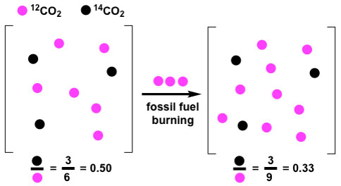
Figure 6 is a schematic illustration of atmospheric CO2 change as CO2 from the combustion of fossil fuels is added. Explain how the figure captures the responses in the previous four items and the results in Figure 5. |
||
|
|||
12.
|
What can you conclude about the origin of the CO2 that has been added to the atmosphere since 1800? Explain the evidence for your reasoning. |
||
D. Atmospheric CO2 from burning fossil fuels: |
|||
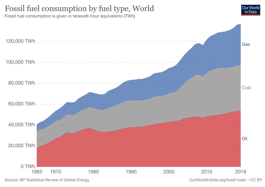
In discussions of global warming and climate disruption, we sometimes forget that burning fossil fuels requires more than just the fuel. Oxygen from the air is an essential reactant and is removed from the air, as it is incorporated into the carbon dioxide product. The fossil fuels burned now are coal and hydrocarbons (natural gas, oil, and gasoline). As a crude model to represent burning equal amounts (moles) of coal and hydrocarbon fuels we can use this reaction. C + CH4 + 3 O2 → 2 CO2 + 2 H2O The rationale for this reaction model are the data in Figure 7 and the combustion enthalpies of carbon, about -400 kJ/mol, and methane, about -800 kJ/mol. Figure 7 shows that about two-thirds of the world’s recent fossil fuel energy comes from oil and gas and one-third from coal. The energy released by the model reaction represents the world’s energy use. Two-thirds of the energy comes from the methane (“oil and gas”) and one-third from carbon (“coal”), which is the ratio for the world in Figure 7. |
|||
|
|||
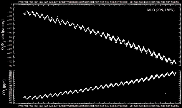
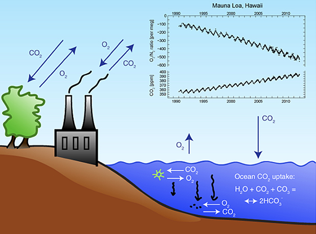
For every two molecules of carbon dioxide formed in our model reaction, three molecules of oxygen react. If the carbon dioxide being added to the atmosphere is from fossil fuel burning, we expect to see the amount of atmospheric oxygen decreasing. This is exactly what the upper curve on the plot in Figure 8 shows. The units on the oxygen concentration axis (upper scale) are equivalent to parts per million molecules of oxygen. The values decrease (oxygen disappears) as carbon dioxide concentration (lower scale) increases. |
|||
|
|||
13.
|
About how large was the decrease in O2 concentration (parts per million molecules O2) from January 1991 to December 2020? Explain your reasoning. What was the average decrease per year for this 30-year period? |
||
14.
|
The atmosphere is about 21% O2 by volume. In 1,000,000 molecules of air, about 210,000 are O2. In item 13 you found the number of O2 molecules out of a million O2 molecules that disappear each year. How many O2 molecules out of 210,000 O2 molecules disappear each year? This is the number of molecules of O2 that disappear per million air molecules, that is, the ppm change in O2. Explain your reasoning. |
||
15.
|
About how large was the increase in CO2 concentration (ppm) during this same 30-year period? Explain your reasoning. What was the average increase per year? |
||
16.
|
About half of the CO2 produced by human activities, mainly fossil fuel burning, remains in the atmosphere each year. If all the CO2 remained in the atmosphere, what would be the increase in concentration (ppm) each year? Show your reasoning. |
||
17.
|
If, for every two CO2 produced each year, three O2 are required from the atmosphere, what should be the decrease in concentration (ppm) of O2 each year? Explain your reasoning. |
||
18.
|
How do the modeled results from item 17 compare to the observed results from item 14? Does the comparison make sense? Explain your reasoning. |
||
19.
|
The sawtooth pattern of the curves in Figure 8 are annual cycles of change in the amounts of CO2 and O2 (superimposed on the long term increase and decrease). The saw teeth in the two curves are complementary. Troughs or low points in the O2 saw teeth occur when the CO2 saw teeth reach their peaks and vice versa. Peaks in CO2 occur in April/May and low points in September/October, in these northern hemisphere data. What do you think causes the annual cycle of change in atmospheric CO2 concentration and what is your evidence? Does this also explain the cyclic change in O2 concentration and why it is offset from the CO2 change? Clearly explain your reasoning. |
||
Appendix A. Mass of atmosphere |
|||
Whenever you read a barometer, you are weighing the atmosphere. The force pressing down on the surface and supporting the column of barometric fluid (usually mercury) is a result of the gravitational attraction by the Earth on the mass of the atmosphere directly above it. For mercury, the height of the barometric column at sea level is 76 cm (= 0.76 m). Imagine a barometer with a tube that has a cross-sectional area of one square meter, 1 m2. The mass of mercury (density = 13.5 x 10³ kg/m3) in this barometric column at sea level is equal to the mass (in kg) of air pressing down on each square meter of Earth’s surface. This barometer column has a volume of 0.76 m3 and, therefore, a mass of 10.3 x 10³ kg/m2. The total mass of the atmosphere is this mass per square meter multiplied by the Earth’s surface area. The radius of the Earth is about 6.4 x 10⁶ m, so, assuming a spherical planet, the surface area is |
|||
 |
|||
| Instructor/presenter notes | |||
Part A |
|||
1.
|
The average mass of a mole of atmospheric gas is 29 g, so the number of moles of gas in 5.3 x 10²¹ g of atmosphere is |
||
2.
|
One ppm (one millionth) of the number of moles of atmospheric gas is 1 ppm atm = (1.8 x 10²⁰ mol)(10-6) = 1.8 x 10¹⁴ mol/ppm |
||
3.
|
The number of moles in 418 ppm of CO2 (or any gas) in the atmosphere is mol CO2 = (418 ppm)( 1.8 x 10¹⁴ mol/ppm) = 7.52 x 10¹⁶ mol |
||
4.
|
One mole of CO2 is 44 g CO2, so 1.8 x 10¹⁴ mol/ppm has a mass of mass 1 ppm CO2 = (44 g/mol CO2)(1.8 x 10¹⁴ mol/ppm) (To make estimations involving ppm atmospheric CO2, it’s often easiest to round to 8 Gt/ppm.) |
||
5.
|
The concentration of CO2 in the atmosphere has grown from about 280 to about 418 ppm since 1800. That is, 138 ppm CO2 has been added to the atmosphere. The mass added is mass added CO2 = (138 ppm)(7.9 Gt/ppm) = 1.09 x 10³ Gt = 1.09 x 10¹⁸ g |
||
Part B |
|||
6.
|
The information about radiocarbon dating indicates that the older the sample, the lower the fraction of 14C it will contain, because of the radioactive decay. Thus, the logical choice is that the data will show increasing amounts (fractions) of 14C, as the tree rings get younger (more recent). A weak case could be made that the time period, about 130 years, is so short compared to the half-life, 5730 years (only about 2% of the half-life), that any change is too small to detect and the fraction will appear unchanged. The information given, however, suggests that the mass spectrometric method is sensitive enough to detect such small changes, so this choice is inconsistent with the ideas presented. On the basis of the previous information in this worksheet, there is no basis for choosing a decreasing trend for the 14C fraction. That’s why the experimental data shown in the succeeding section will be so counterintuitive (perhaps even “counterfactual”) and require rethinking what is happening to the atmosphere. |
||
Part C |
|||
7.
|
From Wikipedia, “A fossil fuel is a fuel formed by natural processes, such as anaerobic decomposition of buried dead organisms, containing energy originating in ancient photosynthesis. The age of the organisms and their resulting fossil fuels is typically millions of years, and sometimes exceeds 650 million years.” We usually think of fossils as remains from past organisms that have been transformed by various chemical and physical processes to some mineralized form—like the fossil shells and so on found in limestone deposits. By analogy, the remains of organisms that died and decayed to coal, oil, and natural gas over millions of years are named as fossils. |
||
8.
|
The carbon in fossil fuels came from the atmosphere millions of years ago and none has been added since. After 100,000 years, about 17 half-lives, only 0.0000076 fraction of the original 14C is left. After a million years, there is no detectable 14C in a fossil fuel. With no 14C in fossil fuels, there is no 14C in the CO2 produced by burning them. That is, about 1.09 x 10³ Gt of CO2(138 ppm) containing no 14C have been added to the atmosphere by fossil-fuel burning. |
||
9.
|
If the cosmic ray flux is about constant, the number of neutrons produced in the atmosphere per unit time will be constant. The amount of nitrogen in the atmosphere has not changed over the past several hundred (perhaps millions) of years. Thus, we expect that the rate of production of 14C will have remained about the same. |
||
10.
|
If the rate of production of 14C remains about the same, we expect that the rate of formation of CO2 containing 14C (formed from the 14C by reaction with oxygen) will remain about the same. The 14C is also continuously decaying, so CO2 containing 14C is continuing to be lost. A steady state is maintained with the rate of formation and rate of decay equal. The number of molecules of CO2 containing 14C will always be about the same over time. (This is, of course, the basic requirement for radiocarbon dating of samples.) |
||
11.
|
The illustration shows addition to the atmosphere of CO2 containing no 14C (from fossil fuel burning, as reasoned in items 7 and 8). It also shows that the number of molecules of CO2 containing 14C remains constant, as reasoned in items 9 and 10. The ratios at the bottom of the illustration show that the proportion of a sample of atmospheric CO2 that contains 14C goes down as CO2 without 14C is added. This is just what the experimental data in Figure 5 show. The continued addition of CO2 since 1800 has diluted the natural abundance of CO2 that contains 14C. |
||
12.
|
It is tempting to conclude that the correlation between lots of fossil fuel burning and increased atmospheric CO2 means the CO2 comes from the burning. But correlation is not necessarily causation. The dilution model illustrated in Figure 6 and described in item 11 explains the data in Figure 5 and provides evidence that the CO2 added to the atmosphere since 1800 comes from fossil fuel burning. Evidence that the added CO2 contains no 14C strengthens the conclusion that fossil fuels are the source of the increased CO2. |
||
Added to the evidence from 14C studies, that fossil fuel burning is the source of added atmospheric CO2, are data from studies on the proportion of the stable isotope 13C in atmospheric CO2, Figure 9. Although the difference between the molecular masses of 13CO2 and 12CO2 is small, most geological and biological reactions that involve CO2 discriminate in favor of one or the other of the isotopic species. What this means is that the products of the reactions have slightly different ratios of 13C/12C than those in the reacting molecules. In particular, the process of photosynthesis favors 12CO2. This means that less 13C is incorporated in the products and the 13C/12C ratio in plant material is lower than that in the atmosphere from which the CO2 came. Since fossil fuels were formed from plant materials, their 13C/12C ratio is low. If CO2 produced by burning fossil fuels is added to the atmosphere, the same sort of dilution discussed above for 14C occurs for 13C, as shown in Figure 9. Beginning in about 1800, the atmospheric proportion of 13CO2 decreases, as atmospheric CO2 increases, after both have been essentially constant for the previous 800 years. |
|||
|
|||
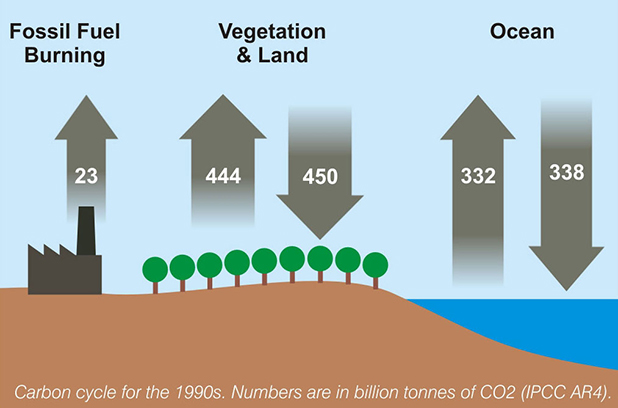
Analysis of data like those in Figures 5 and 9, is not as straightforward as the simple dilution model in Figure 6. The flux of CO2 from its various sinks and sources is enormous. As the simple graphic, Figure 10, indicates, a great deal of exchange occurs that must be considered to account for the actual numerical values in Figures 5 and 9. Here we have looked at the forest. The trees have to wait for deeper dives into climate science than makes sense for a beginning look. |
|||
|
|||
Part D |
|||
13. |
The oxygen concentration per million oxygen molecules decreases from about –100 ppm to about –700, approximately 600 ppm change in 30 years, or about 20 ppm O2 per year.
|
||
14. |
Multiply the number of oxygen molecules per million molecules in the atmosphere by the fraction of oxygen molecules that disappear each year to get the number of oxygen molecules per million air molecules that disappear. It’s important to recognize that this is a trace amount of O2 loss and we are in no danger of “using up” our atmospheric O2 in combustion reactions. On the other hand, adding further “trace” amounts of combustion product greenhouse gases will exacerbate the already disastrous disruption of the climate. |
||
15. |
The carbon dioxide concentration increases from about 355 ppm to about 415 ppm in 30 years, approximately 60 ppm change, or about 2.0 ppm per year.
|
||
16. |
If 2.0 ppm/yr from item 15 represents only half the carbon dioxide produced by fossil fuel burning, the total amount would be equivalent to 4.0 ppm/yr.
|
||
17. |
From the stoichiometry, (3 O2 react)/(2 CO2 formed), we find the amount of O2 lost,
|
||
From item 2 for the relationship of moles to ppm in the atmosphere, we find the moles of O2 lost, (6.0 ppm O2 lost/yr)(1.8 x 1014 mole/ppm) Go to the FAQ page at scrippso2.ucsd.edu for more information on oxygen, carbon dioxide, fossil fuels, etc., where you find, “The annual global O2 consumption from fossil-fuel burning in year 2005 was 917 Tmol O2 or 9.17×10¹⁴ moles of O2.” This value was calculated from more extensive data about the actual amounts of each fossil fuel burned and oxygen consumption for each kind. It may be fortuitous that the value calculated here for a crude model is within about 15% of the value on the website, but it’s evidence that the model is not wholly bogus. These correlations and quantitative relationships between the increase in atmospheric carbon dioxide and decrease in atmospheric oxygen are further evidence that it is fossil fuel burning that adds atmospheric greenhouse gas, which causes global warming and climate disruption. |
|||
18. |
Less net oxygen is lost from the atmosphere (4.0 ppm/yr) than is required to react with all the fossil fuels that are burned (6.0 ppm/yr, based on the amount of carbon dioxide added to the atmosphere). The simplest explanation is that some oxygen is being added to the atmosphere as it is also being used up for combustion, Figure 11.
|
||
|
|||
The major source of atmospheric oxygen on Earth is photosynthesis, from land, represented on the far left of Figure 11, and from the sea, shown as O2 from the ocean in the figure. Photosynthesis harnesses the energy of light to drive the formation of carbohydrates [general formula, C(H2O), “carbon hydrate”] from carbon dioxide and water, CO2 + H2O + light → C(H2O) + O2 (This expression can be a bit misleading. The O2 produced by photosynthesis comes from the oxygen atoms in the water and this is not at all obvious from this expression.) The conclusion that might be drawn is that, with extra carbon dioxide available, more photosynthesis occurs than normally would occur. This would put oxygen that had reacted to form carbon dioxide back into the air, so not as much would disappear. In parallel with the production of oxygen, the amount of plant material (result of the additional carbohydrate) on Earth should increase. Satellites observing vegetation have shown that the Earth has been “greening” over the past decades, which is consistent with more plant growth. Whether this effect will continue as the temperature continues to climb, no one knows. This is an example of the sort of uncertainty we live with in a climate-disrupted world. |
|||
19. |
The timing of the cycle for carbon dioxide concentration provides a clue to explain the sawtooth pattern of the Keeling curve. In the northern hemisphere, carbon dioxide goes annually from its highest value in the spring to its lowest value in the fall. This is summer, the growing season for crops and plants of all kinds. Plant growth means lots of photosynthesis and, hence, a large need for carbon dioxide to incorporate into carbohydrates. Thus, carbon dioxide concentration in the atmosphere goes down in the summer. During the winter, there is less growth. The processes of decay, which produce carbon dioxide, predominate and add carbon dioxide to the atmosphere. When photosynthesis is at its peak in the summer, oxygen is being produced, so its concentration grows while carbon dioxide declines. The opposite occurs in the winter, when oxygen is used up in decay of organic matter that produces carbon dioxide. |
||
Natural processes producing and using carbon dioxide are actually fairly delicately balanced, as you can see by comparing the size of the saw teeth in the Keeling curve, Figure 1, with the large fluxes shown in Figure 10. The maximum to minimum change for each annual cycle in the Keeling curve is about 7 ppm. From item 4 above, 1 ppm atmospheric CO2 = 7.9 Gt CO2, so the annual variation is about 55 Gt [= (7 ppm)( 7.9 Gt/ppm)]. The annual flux between the surface (land and sea) and atmosphere shown in Figure 10 involves about 800 Gt CO2, almost 15 times larger. Thus, the seasonal imbalance between natural processes producing and using carbon dioxide does not seem to exceed about seven percent. |
|||
|
|||
To obtain a Word file of this Activity, please fill out this brief form to help us track what is happening to our Workbook. We also encourage you to get in touch if you have an activity or idea for an activity that might add to the Workbook. We want to make this an alive and active document. |
|||
 |