Temperature, water volume, and sea level
|
Temperature, water volume, and sea level |
Water in the oceans acts as a high-heat-capacity energy buffer to prevent massive swings in Earth’s temperature from day to night and from season to season. And oceans absorb most of the extra energy trapped by increased atmospheric greenhouse gases from fossil fuel burning and other human activities, which puts the brakes on global surface warming. As the oceans gain this energy, they warm. To understand the consequences of a warming sea, we will investigate the effect of temperature on a mass of water and relate the results to the oceans. |
||||
|
||||
| Procedure | ||||
Plan an experiment to measure the volume change of a known volume of cool water when you warm it a few degrees. Keep in mind that the change will be a small fraction of the volume of the water, so you will need a lot of water and a way to measure a small volume change. Check your plan with one of the instructors to be sure it is safe and likely to provide the data needed to calculate the thermal coefficient of change, that is, the decimal fraction of volume change of water per degree change in temperature. It may be useful to know that the density of liquid water in the 10-20 °C temperature range is 1.00 g·mL–1. When your plan (or an amended version, if necessary) is approved, carry it out and find the thermal coefficient of change for water. |
||||
Analysis |
||||
1.
|
Does the volume of water expand, contract, or stay the same as the temperature increases? Clearly explain the evidence for your answer. What do you think is happening at the molecular level to account for your observations? |
|||
2.
|
What was the exact (±1 mL) volume of water you used? Clearly describe how you determined this value. |
|||
3.
|
What was the temperature change for your water sample? Clearly explain how you brought about this change and what temperatures you measured. |
|||
4.
|
What was the volume change for your water sample? Clearly describe how you determined this value and all the measurements you made. |
|||
5.
|
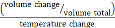
From the results in items 2, 3, and 4, the total volume of water and its volume change per degree are known. Calculate the coefficient of thermal expansion (or contraction, if the volume is decreasing), that is, the decimal fraction of change in volume per degree temperature change. coefficient of thermal expansion of water = __________ |
|||
6.
|
The Earth is approximately a large sphere with a surface area of about 5 x 10¹⁴ m2, which is about 70% covered in seawater. Estimate the volume of the top 300 m of the Earth’s oceans. Explain any assumptions you make to get this estimate. |
|||
7.
|
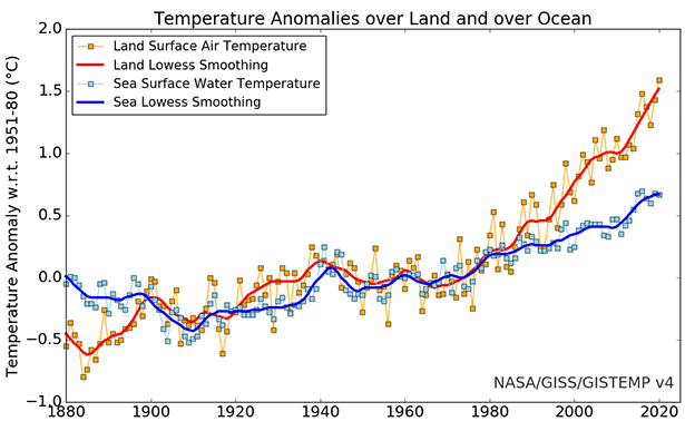
The graph, Figure 1, from NASA shows the observed changing land and sea surface temperatures since the mid-20th century. What has been the change in sea surface temperature (smooth blue curve) from 1993 to 2020? Explain the reasoning for your response. |
|||
|
||||
8.
|
Assume that rise in sea surface temperature is also reflected in the rise of the temperature of the top 300 m of the oceans. Use the thermal expansion coefficient you determined to find the increase in volume of the top 300 m of the oceans due to the warming during the 1993 to 2020 period. What assumption(s) do you need to make? Explain your reasoning clearly. |
|||
9.
|
How much sea level rise will the thermal volume increase in item 8 cause? Explain your reasoning clearly. |
|||
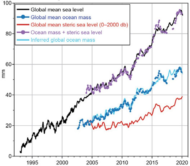
10.
|
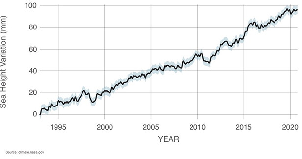
Figure 2 shows the rise in mean (average) sea level from 1993 through 2020. What was the increase in average sea level during this period? How does your calculation of the sea level rise from item 9 compare to this observed change? How might you account for any difference between calculation and observation? Explain your reasoning clearly. |
|||
|
||||
An extension |
||||
From 1994 to 2017 the warming Earth lost 28,000,000,000,000 (28 trillion) metric tonnes of ice. This is the conclusion of a 2020 preprint for discussion “Review Article: Earth’s ice imbalance”, by Slater, T., Lawrence, I. R., Otosaka, I. N., Shepherd, A., Gourmelen, N., Jakob, L., Tepes, P., & Gilbert, L. in The Cryosphere. Here is the abstract for this review. |
||||
|
We combine satellite observations and numerical models to show that Earth lost 28 trillion tonnes of ice between 1994 and 2017. Arctic sea ice (7.6 trillion tonnes), Antarctic ice shelves (6.5 trillion tonnes), mountain glaciers (6.2 trillion tonnes), the Greenland ice sheet (3.8 trillion tonnes), the Antarctic ice sheet (2.5 trillion tonnes), and Southern Ocean sea ice (0.9 trillion tonnes) have all decreased in mass. Just over half (60 %) of the ice loss was from the northern hemisphere, and the remainder (40 %) was from the southern hemisphere. The rate of ice loss has risen by 57 % since the 1990s – from 0.8 to 1.2 trillion tonnes per year – owing to increased losses from mountain glaciers, Antarctica, Greenland, and from Antarctic ice shelves. During the same period, the loss of grounded ice from the Antarctic and Greenland ice sheets and mountain glaciers raised the global sea level by 35.0 ± 3.2 mm. The majority of all ice losses were driven by atmospheric melting (68 % from Arctic sea ice, mountain glaciers, ice shelf calving, and ice sheet surface mass balance), with the remaining losses (32 % from ice sheet discharge and ice shelf thinning) being driven by oceanic melting. Altogether, the cryosphere has taken up 3.2 % of the global energy imbalance. |
|||
11.
|
What volume of water (in m3) is required to raise global sea level by one millimeter (10-3 m)? |
|||
12.
|
How many of the 28 trillion tonnes of ice melt water caused sea level rise? Carefully explain the reasoning for your response. |
|||
13.
|
One tonne of water occupies a volume of one cubic meter. How many cubic meters of water did the ice melt from item 12 add to the seas between 1994 and 2017? What was the sea level rise (in millimeters) caused by this ice melt water? Explain your reasoning. |
|||
14.
|
Does the result in item 13 help to understand the observations in item 10 and Figure 2? Explain why or why not. |
|||
 |
||||
Instructor/presenter notes |
||||
The key to good results in this activity is to seal the flask full of water (no air bubble at the top) with the stopper in a way that forces water a couple centimeters into the graduated measuring pipet inserted in the stopper. Some variant of this procedure should be satisfactory. Weigh the dry flask and stopper assembly (stopper, pipet, and thermometer) empty and fill with water to the very top. Insert the stopper, being careful not to trap any air, but allowing water to overflow as necessary, and driving water into the pipet, as the stopper seals. The liquid level in the pipet should be 2-3 cm above the stopper to be easy to read. (You might have available a long-stem plastic pipet with an attached length of small diameter tubing to remove water from pipets that are too full.) Dry off the flask and reweigh it filled with water to get the mass of water (to be converted to volume). Record the temperature of the liquid in the flask and volume reading of the liquid in the pipet. Warm the water-filled flask for a few minutes on a hot plate (or mug warmer) and then let it sit until the temperature is constant. Record the new temperature and volume reading of liquid in the pipet. If necessary, repeat the heating until at least one milliliter of liquid has entered the pipet. The initial and final temperature and pipet volume readings can be used to calculate the coefficient of thermal expansion. If more than one temperature and volume reading is made, the values can be plotted to get a slope that could be more accurate than using just the end points, but is unnecessary to get usable results. This activity could also be done “in reverse” by starting with water just above room temperature and adding water to the pipet, as necessary, to bring the volume reading near zero and then making temperature and volume measurements as the water cools. The pedagogical problem with this technique is that it focuses on contraction, but the climate connection is to sea level rise due to rising temperature and thermal expansion. The absolute numerical values for the coefficients of expansion and contraction are identical, of course, but with opposite signs. It just seems more straightforward to do the “modeling” in the same direction (increasing temperature) as the system to which it is applied. |
||||
1. |
This first question is included to direct students simply to think directionally about their results and propose a model to explain the direction before getting bogged down in calculations. The rising column of water in the pipet shows that the liquid volume must be increasing to add volume to the pipet as the temperature increases. (The small change in volume in the pipet compared to the large volume in the flask can also be reprised when the sea level rise is calculated later.) As temperature increases, molecular motion increases and the molecules get, on the average, a bit farther apart. Thus, the volume increases (and density decreases)—the liquid has undergone thermal expansion. It’s not necessary to know anything in particular about the structure and interaction of the molecules to do this reasoning. (Similar reasoning is applied in the Density and behavior of ice-water mixtures to explain the sinking of ice cold water in room temperature water.) |
|||
2. |
The mass of water in the apparatus should be a little more than 500 g (since the flask filled to the rim holds a bit more than 500 mL), which gives a volume of a little over 500 mL when mass is divided by 1.00 g/mL. |
|||
3. |
Waiting until the temperature is constant after heating is important to help assure that the entire volume has reached the same temperature. This can take a fair amount of time for a large volume of water. |
|||
4. |
The volume change measured in the pipet is the difference between the initial and final volume readings, remembering to read as though water is being delivered from the pipet. (The volume change is initial minus final reading, because the change is positive, but the pipet is being read "in reverse".) The coefficient of thermal expansion of water is 2.1 x 10⁻⁴ K-1. For a 10 °C (= 10 K) rise in temperature, the fractional change in water volume is (2.1 x 10⁻⁴ K-1)(10 K) = 2.1 x 10⁻³. If all goes well in this activity, we expect a volume change of about (500 mL)(2.1 x 10⁻³) ≈ 1 mL for a 10 °C increase in temperature. This water would be forced into the pipet and should be readily measurable. |
|||
5. |
The coefficient of thermal expansion is calculated as |
|||
The rest of the questions in the worksheet are designed to drive home the idea that thermal expansion and the coefficient of thermal expansion apply to any volume of water, no matter how large, and in particular to sea level rise in a warming world. Possible responses to the items are: |
||||
6. |
The area of the surface covered by the oceans is 0.70 (5 x 10¹⁴ m2) = 3.5 x 10¹⁴ m2. The volume of the top 300 m layer of the ocean is (3.5 x 10¹⁴ m2) (300 m) = 1.05 x 10¹⁷ m3. This calculation assumes that the ocean is at least 300 m deep right up to the shores of the continents. This is not true, of course, but the oceans are so vast that the “error” is negligible for the simple calculations we are making here. We are also ignoring the curvature of the Earth, which makes the lower boundary of the 300 m a bit smaller in area than the surface layer. |
|||
7. |
Although the plot is a bit difficult read, the sea surface temperature anomaly in 1993 was about 0.25 °C and rose to about 0.70 °C by 2020, an increase of 0.45 °C (0.45 K). |
|||
8. |
The increase in volume of the top 300 m of ocean from 1993 to 2020 (with the accepted coefficient of thermal expansion of water value in place of the one that will be measured in this Activity) is ΔV = (1.05 x 10¹⁷ m3) (2.1 x 10⁻⁴/K) (0.45 K) = 9.9 x 10¹² m3 This approach assumes that the coefficient of thermal expansion measured for pure water can be applied to sea water. Students should look up the value for sea water to see how appropriate this assumption is. Another possibility is to do the activity with sea water (or have some groups do it with sea water to compare with pure water). A mix of salts is available in pet stores for making “sea water” for marine aquaria. |
|||
9. |
Accounting for this increase in volume is like adding a thin layer on top of the 300 m layer. This layer would have a surface area = 3.5 x 10¹⁴ m2, so its depth would be its volume divided by the surface area. |
|||
10. |
The satellite data from 1993 to 2020 show a sea level rise of about 95 mm. Compared to this calculated value, 28 mm, from thermal expansion, this is a discrepancy of a factor of three. Where does the rest of the water come from? The vast ice sheets on Greenland and Antarctica and glaciers around the world are melting as the Earth warms. All that thawed ice ends up in the oceans, where it raises the sea level by adding volume. So, there are two major contributions to sea level rise in a climate disrupted world—thermal expansion and addition of new water, as demonstrated in the Extension related to Earth’s ice melt. |
|||
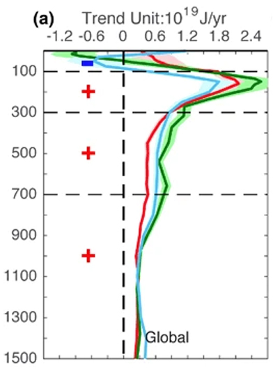
A possible alternative argument for the discrepancy could be that the choice of 300 m for the depth of warming that is like the surface is incorrect and it should be deeper. If it was three times deeper, the thermal expansion calculation would give a value close to 84 mm. A rationale for choosing 300 m (or at least a depth not hugely different) is provided by the data in Figure 3. The plot shows that the rate of energy absorption by the oceans, number of joules per year as a function of depth during the past two decades, has been greatest in the first 300 m and drops off significantly at greater depths. This means that most of the recent warming has occurred in this layer. Over decades and centuries, energy from the top layers will be mixed into deeper and deeper layers. The massive convection currents (“conveyor belts” carrying water throughout the globe) that bring surface water to the very bottom of the oceans (and vice versa) take millennia to make the journey. Only a tiny amount of global warming has yet made it to the abyssal waters. (See Heat capacity and fate of Earth’s energy imbalance for more on the Earth’s energy gain.) |
||||
|
||||
Extension |
||||
11. |
The volume of a one millimeter layer of water on top all the seas of the planet is given by the product of the surface area of the seas (3.5 x 10¹⁴ m2) and the depth of the layer (10-3 m). volume of 1 mm ocean layer = (3.5 x 10¹⁴ m2) (10-3 m) |
|||
12. |
Melted ice water that was originally ice on land adds volume to the oceans, that is, the vast ice sheets on Greenland and Antarctica and glaciers around the world. (See Density and behavior of ice-water mixtures for experimental evidence that water from floating ice does not add to the liquid level.) The abstract gives the contributions as Greenland ice sheet, 3.8 trillion tonnes, glaciers, 6.2 trillion tonnes, and Antarctica ice sheet, 2.5 trillion tonnes, for a total of: |
|||
13. |
Since a tonne of water is a cubic meter of water, a teratonne of water is a trillion cubic meters (1 x 10¹² m3). Therefore, 12.5 Tt water is 12.5 x 10¹² m3 of water. The depth of the layer this volume of water will add to the oceans is this volume divided by the volume of a 1 mm layer. |
|||
| 14. | The result in item 13 added to the thermal expansion result in item 9 (28 mm), gives a total of 64 mm of sea level rise between the late 20th century and about 2017, which is more in the ballpark of the observed 95 mm rise, Figure 2. It appears that melting ice from the land and thermal expansion, both the result of a climate disrupted warming world, are contributing comparable amounts to the sea level rise that is threatening coastal communities. | |||
Some added information might be gleaned from the data in Figure 4. The black curve that begins in 1993 shows the same satellite data for mean sea level as in previous Figure 2. The various satellites that collected those data have spanned the entire planet and provide an excellent view of one of the ways it’s changing as it warms. |
||||
|
||||
The data for the red curve here (and those in Figure 3 above) are from a fleet of about 3500-4000 Argo floats distributed throughout the oceans since 2005. These floats sink to a depth of 2000 meters and then periodically rise slowly to the surface taking readings of temperature and salinity (saltiness) as a function of depth. When they reach the surface, they send their GPS coordinates and the recorded data to a satellite for transmission to the laboratories where the information is stored and analyzed. Then the floats sink again to repeat the process. The floats last about three years and about 1000 or more are added each year to maintain the coverage of the oceans. (Argo float data are also referenced in Heat capacity and fate of Earth’s energy imbalance.) From this large amount of data, the thermal expansion of the seas can be calculated more precisely than from our simple model. (The figure legend calls this the “steric sea level”. “Steric” refers to the spatial arrangement of the water molecules. In this case, that means the distance between them, which increases as the sea warms and expands.) The value in 2020 was about 37 mm, which corresponds reasonably well with our simple calculation of 28 mm, and gives some confidence in our approach. The data for the blue curve in the figure are derived from the global mean change in the ocean mass. One kilogram of water is essentially one liter of water, so converting mass change to volume change is straightforward and then sea level rise is calculated as we did. Sea water is only two to three percent more dense than pure water, so little correction is necessary to account for the difference. Weighing the ocean is done by a pair of NASA satellites, the Gravity Recovery and Climate Experiment (GRACE) mission, measuring changes in gravity over the entire Earth since 2002. (Substitution by a replacement pair of satellites, GRACE-Follow-On (GRACE-FO), explains the small gap in data in 2018. There is reference to other GRACE data in Density and behavior of ice-water mixtures.) The 2016-2017 value is about 50 mm, which is quite a bit higher than the item 13 calculated value, 36 mm, for added ice melt from land ice. It seems there might be some other source of the added water. One possibility is ice melt from the Antarctic ice shelves. Ice shelves are enormous tongues of ice that extend into the ocean at the leading edge of coastal glaciers and retard the flow of the glaciers toward the sea. At least part of an ice shelf is generally “grounded”, which means that all or part of it is sitting on the sea floor and not floating, so its melt adds to ocean volume. The parts that are not sitting on the sea floor are exposed to warming sea water beneath the shelf that melts it away. The abstract about global ice loss says that the shelves are thinning because of this action. We found that the loss of 12.5 Tt of ice accounts for a 36 mm sea level rise. To get a further 14 mm rise would require an ice melt of (14/36) (12.5 Tt ice) ≈ 5 Tt ice. The abstract indicates that the shelves have lost 6.5 Tt of ice, which, according to this calculation, could be the source of the sea level rise not accounted for by land ice melt. And the ice shelves are in trouble: Lhermitte, S., Sun, S., Shuman, C., Wouters, B., Pattyn, F., Wuite, J., Berthier, E., & Nagler, T., Damage accelerates ice shelf instability and mass loss in Amundsen Sea Embayment [West Antarctic ice shelf], Proceedings of the National Academy of Sciences, 2020, 117 (40), 24735-24741. Here is another observation about melting ice and sea level that can be treated the same way as the information on Earth’s total ice melt and yields a satisfying conclusion. |
||||
| Chain reaction of fast-draining lakes poses new risk for Greenland ice sheet “This growing network of melt lakes, which currently extends more than 100 kilometres inland and reaches elevations as high a 2,000 metres above sea level, poses a threat for the long-term stability of the Greenland ice sheet,” said lead author Dr. Poul Christoffersen, from Cambridge’s Scott Polar Research Institute. “This ice sheet, which covers 1.7 million square kilometres, was relatively stable 25 years ago, but now loses one billion tonnes of ice every day. This causes one millimetre of global sea level rise per year, a rate which is much faster than what was predicted only a few years ago.” Source: University of Cambridge, “Chain reaction of fast-draining lakes poses new risk for Greenland ice sheet,” ScienceDaily, 14 March 2018. Reference: Christoffersen, P., Bougamont, M., Hubbard, A., Doyle, S. H., Grigsby, S., & Pettersson, R., “Cascading lake drainage on the Greenland Ice Sheet triggered by tensile shock and fracture.” Nature Communications (2018). |
||||
|
||||
To obtain a Word file of this Activity, please fill out this brief form to help us track what is happening to our Workbook. We also encourage you to get in touch if you have an activity or idea for an activity that might add to the Workbook. We want to make this an alive and active document. |
||||
| Back to Table of Contents | ||||
 |